Its very common, The GROUP BY statement to is used to summarize data, is almost as old as SQL itself. Microsoft introduced additional paradigm of ROLLUP and CUBE to add power to the GROUP BY clause in SQL Server 6.5 itself. The CUBE or ROLLUP operators, which are both part of the GROUP BY clause of the SELECT statement and The COMPUTE or COMPUTE BY operators, which are also associated with GROUP BY.
A very new feature in SQL Server 2008 is the GROUPING SETS clause, which allows us to easily specify combinations of field groupings in our queries to see different levels of aggregated data.
These operators generate result sets that contain both detail rows for each item in the result set and summary rows for each group showing the aggregate totals for that group. The GROUP BY clause can be used to generate results that contain aggregates for each group, but no detail rows.
COMPUTE and COMPUTE BY are supported for backward compatibility. The ROLLUP operator is preferred over either COMPUTE or COMPUTE BY. The summary values generated by COMPUTE or COMPUTE BY are returned as separate result sets interleaved with the result sets returning the detail rows for each group, or a result set containing the totals appended after the main result set. Handling these multiple result sets increases the complexity of the code in an application. Neither COMPUTE nor COMPUTE BY are supported with server cursors, and ROLLUP is. CUBE and ROLLUP generate a single result set containing embedded subtotal and total rows. The query optimizer can also sometimes generate more efficient execution plans for ROLLUP than it can for COMPUTE and COMPUTE BY. When GROUP BY is used without these operators, it returns a single result set with one row per group containing the aggregate subtotals for the group. There are no detail rows in the result set.
To demonstrate all these, lets create a sample table as SalesDate as
— Create a Sample SalesData table
CREATE TABLE SalesData (EmpCode Char(5), SalesYear INT, SalesAmount MONEY)
— Insert some rows in SaleData table
INSERT SalesData VALUES(1, 2005, 10000),(1, 2006, 8000),(1, 2007, 17000),
(2, 2005, 13000),(2, 2007, 16000),(3, 2006, 10000),
(3, 2007, 14000),(1, 2008, 15000),(1, 2009, 15500),
(2, 2008, 19000),(2, 2009, 16000),(3, 2008, 8000),
(3, 2009, 7500),(1, 2010, 9000),(1, 2011, 15000),
(2, 2011, 5000),(2, 2010, 16000),(3, 2010, 12000),
(3, 2011, 14000),(1, 2012, 8000),(2, 2006, 6000),
(3, 2012, 2000)
ROLLUP : – The ROLLUP operator generates reports that contain subtotals and totals. The ROLLUP option, placed after the GROUP BY clause, instructs SQL Server to generate an additional total row. Let see the examples as per our TestData from SalesData Table.
Select EmpCode,sum(SalesAmount) as SalesAMT from SalesData Group by ROLLUP(EmpCode)
Will show result as ,

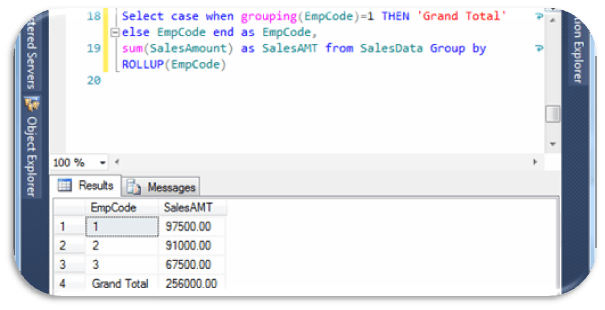
Here we can see clearly sum of all EmpCode with NULL title, Once a guy asked about this NULL , How to give Name for this Null as suppose ‘Grand Total’, here is some manipulation with tricky tips and we can get the desired output and we can also change it as where its required.
Select
case when grouping(EmpCode)=1 THEN ‘Grand Total’ else EmpCode end as EmpCode,
sum(SalesAmount) as SalesAMT from SalesData Group by ROLLUP(EmpCode)
will show result as,
In ROLLUP parameter we can also set multiple grouping set like ROLLUP(EmpCode,Year), hence ROLLUP outputs are hierarchy of values as per selected columns.
CUBE : The CUBE operator is specified in the GROUP BY clause of a SELECT statement. The select list contains the dimension columns and aggregate function expressions. The GROUP BY specifies the dimension columns by using the WITH CUBE keywords. The result set contains all possible combinations of the values in the dimension columns, together with the aggregate values from the underlying rows that match that combination of dimension values. CUBE generates a result set that represents aggregates for all combinations of values as per the selected columns. Let see the examples as per our TestData from SalesData Table.
Select EmpCode,SalesYear,sum(SalesAmount) as SalesAMT from SalesData Group by CUBE(SalesYear,EmpCode)
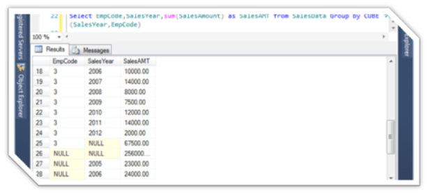
Will shows as
Select SalesYear,EmpCode,sum(SalesAmount) as SalesAMT from SalesData Group by CUBE(SalesYear,EmpCode)
Will show as,
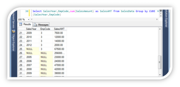
The ROLLUP and CUBE aggregate functions generate subtotals and grand totals as separate rows, and supply a null in the GROUP BY column to indicate the grand total.
the difference between the CUBE and ROLLUP operator is that the CUBE generates a result set that shows the aggregates for all combinations of values in the selected columns. By contrast, the ROLLUP operator returns only the specific result set.The ROLLUP operator generates a result set that shows the aggregates for a hierarchy of values in the selected columns. Also, the ROLLUP operator provides only one level of summarization
GROUPING SETS : The GROUPING SETS function allows you to choose whether to see subtotals and grand totals in your result set. Its allow us versatility as
- include just one total
- include different levels of subtotal
- include a grand total
- choose the position of the grand total in the result set
Let See examples,
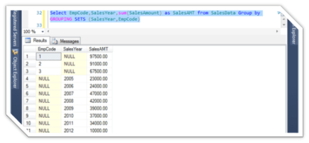
Select EmpCode,SalesYear,sum(SalesAmount) as SalesAMT from SalesData Group by GROUPING SETS (SalesYear,EmpCode)
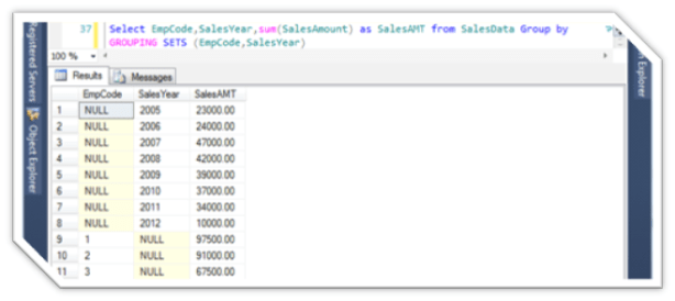
Select EmpCode,SalesYear,sum(SalesAmount) as SalesAMT from SalesData Group by GROUPING SETS (EmpCode,SalesYear)
COMPUTE & COMPUTE BY: The summary values generated by COMPUTE appear as separate result sets in the query results. The results of a query that include a COMPUTE clause are like a control-break report. This is a report whose summary values are controlled by the groupings, or breaks, that you specify. You can produce summary values for groups, and you can also calculate more than one aggregate function for the same group.
When COMPUTE is specified with the optional BY clause, there are two result sets for each group that qualifies for the SELECT:
- The first result set for each group has the set of detail rows that contain the select list information for that group.
- The second result set for each group has one row that contains the subtotals of the aggregate functions specified in the COMPUTE clause for that group.
When COMPUTE is specified without the optional BY clause, there are two result sets for the SELECT:
- The first result set for each group has all the detail rows that contain the select list information.
- The second result set has one row that contains the totals of the aggregate functions specified in the COMPUTE clause.
Comparing COMPUTE to GROUP BY
To summarize the differences between COMPUTE and GROUP BY:
- GROUP BY produces a single result set. There is one row for each group containing only the grouping columns and aggregate functions showing the subaggregate for that group. The select list can contain only the grouping columns and aggregate functions.
-
COMPUTE produces multiple result sets. One type of result set contains the detail rows for each group containing the expressions from the select list. The other type of result set contains the subaggregate for a group, or the total aggregate for the SELECT statement. The select list can contain expressions other than the grouping columns or aggregate functions. The aggregate functions are specified in the COMPUTE clause, not in the select list.
Let See example
Select EmpCode,SalesYear,SalesAmount from SalesData order by EmpCode,SalesYear COMPUTE SUM(SalesAmount)
The COMPUTE and COMPUTE BY clauses are provided for backward compatibility. Instead, use the following components, both are discontinued from SQL Server 2012.