Locking is a means of not allowing any other transaction to take place when one is already in progress. In this the data is locked and there won’t be any modification taking place till the transaction either gets successful or it fails. The lock has to be put up before the processing of the data whereas Multi-Versioning is an alternate to locking to control the concurrency. It provides easy way to view and modify the data. It allows two users to view and read the data till the transaction is in progress. Multiversion concurrency control is described in some detail in the 1981 paper “Concurrency Control in Distributed Database Systems” by Philip Bernstein and Nathan Goodman.
Multi-Versioning, As the name implies, each record in the system might have multiple versions visible to different transactions. When a transaction modifies a record, a new version is written to the database, and a previous version, representing only the difference between the version of the record that was read by the transaction and the new value of the record, is written as a back version of that record.
Read committed isolation using row versioning is somewhere in between Locks and Multi-Versioning. Under this isolation level, read operations do not acquire locks against the active live data. However, with update operations the process is the same for this isolation level as it is for the default read committed isolation level, The selection of rows to update is done by using a blocking scan where an update lock is taken on the data row as data values are read.
Snapshot isolation uses purely Multi-Versioning because data that is to be modified is not actually locked in advance, but the data is locked when it is selected for modification. When a data row meets the update criteria, the snapshot transaction verifies that the data has not been modified by another transaction after the snapshot transaction started. If the data has not been modified by another transaction, the snapshot transaction locks the data, updates the data, releases the lock, and moves on. If the data has been modified by another transaction, an update conflict occurs and the snapshot transaction rolls back.
Although locking can be the best concurrency-control choice for applications that require data consistency and inter-transaction protection, it can cause writers to block readers. If a transaction changes a row, another transaction cannot read the row until the writer commits. There are cases where waiting for the change to complete is the correct response; however, there are cases where the previous transactionally consistent state of the row is enough.
Author Archive
Locking v/s Multi-Versioning
Posted: December 7, 2012 by Virendra Yaduvanshi in Database AdministratorTags: Deadlock, Difference between Locking and Multi Versioning, Isolation Level, Locking, Locking and Multi-Versioning, Locking v/s Multi-Versioning, Multi Version, Read committed, Record Multi-Version, Row Multi version, SQL Server
Reducing BLOCKING and DEADLOCKING issues
Posted: December 4, 2012 by Virendra Yaduvanshi in Database AdministratorTags: Block, Blocking in SQL Server, Deadlocks in SQL Server, Improve SQL Server Performance, Locks, Performance enhancement, RCSI, Read-Committed Snapshot Isolation level, Reducing blocking and deadlocking issues, SQL Server, Transaction, Transaction level isolation
As we know blocking occurs when one SPID holds a lock on a specific resource and a second SPID attempts to acquire a conflicting lock type on the same resource. Typically, the time frame for which the first SPID locks the resource is very small. When it releases the lock, the second connection is free to acquire its own lock on the resource and continue processing. This is normal behavior and may happen many times throughout the course of a day with no noticeable effect on system performance.
By using the read-committed snapshot isolation level introduced in Microsoft SQL Server 2005, we can reduce blocking and deadlocking issues caused by lock contention.Every time a row is modified by a specific transaction, the instance of the Database Engine stores a version of the previously committed image of the row in tempdb.
As per BOL, The read-committed snapshot isolation level provides the following benefits:
- SELECT statements do not lock data during a read operation. Read transactions do not block write transactions and vice versa.
- Since SELECT statements do not acquire locks in most cases, the number of locks required by a transaction is reduced, which reduces the system overhead required to manage locks.
- The possibility of blocking is significantly reduced.
- SELECT statements can access the last committed value of the row while other transactions are updating the row without getting blocked.
- The number of blocks and deadlocks is reduced.
- Fewer lock escalations occur.
A quick and easy way to remember how Read-Committed Snapshot Isolation works:
- Readers DO NOT block Writers
- Writers DO NOT block Readers
- Writers DO block Writers
REMEMBER: TempDB is a critical resource for the performance of Read-Committed Snapshot Isolation. RCSI puts a copy of the records that are being modified in TempDB before the transaction is committed so you need to make sure that TempDB has appropriate space and is placed on fast drives that ideally are isolated away from your user database data and log files.
The default Syntax is as
SET TRANSACTION ISOLATION LEVEL
{ READ COMMITTED | READ UNCOMMITTED | REPEATABLE READ | SERIALIZABLE }
Running Queries Details
Posted: November 28, 2012 by Virendra Yaduvanshi in Database AdministratorTags: Advance SP_WHO, Advance SP_WHO2, Advance version of SP_WHO, Advance version of SP_WHO2, Blocked By, current command, current Query, current running query, Database Administrator, DBA, HOST IP, HOST NAME, Running Queries Details, seeing current running command, SP_who, SP_WHO2, SQL Server, Whats goin on server
As we know, to check whats going on at server level, we commonly use SP_WHO or SP_WHO2 but from both of these, there are no clear picture about exact commands which currently running on server, these shows the command, not exact full text string that’s currently running, Here is a some DMV’s manipulation to find the same.
SELECT SPID = er.session_id
,BlkBy = er.blocking_session_id
,ElapsedMS = er.total_elapsed_time
,CPU = er.cpu_time
,IOReads = er.logical_reads + er.reads
,IOWrites = er.writes
,Executions = ec.execution_count
,CommandType = er.command
,ObjectName = OBJECT_SCHEMA_NAME(qt.objectid,dbid) + ‘.’ + OBJECT_NAME(qt.objectid, qt.dbid)
,SQLStatement = SUBSTRING(qt.text,er.statement_start_offset/2,
(CASE WHEN er.statement_end_offset = –1 THEN LEN(CONVERT(nvarchar(MAX), qt.text)) * 2 ELSE
er.statement_end_offset END – er.statement_start_offset)/2)
,Status = ses.status
,[Login] = ses.login_name
,Host = ses.host_name
,DBName = DB_Name(er.database_id)
,LastWaitType = er.last_wait_type
,StartTime = er.start_time
,Protocol = con.net_transport
,transaction_isolation =CASE ses.transaction_isolation_level
WHEN 0 THEN ‘Unspecified’
WHEN 1 THEN ‘Read Uncommitted’
WHEN 2 THEN ‘Read Committed’
WHEN 3 THEN ‘Repeatable’
WHEN 4 THEN ‘Serializable’
WHEN 5 THEN ‘Snapshot’
END
,ConnectionWrites = con.num_writes
,ConnectionReads = con.num_reads
,ClientAddress = con.client_net_address
,Authentication = con.auth_scheme
FROM sys.dm_exec_requests er
LEFT JOIN sys.dm_exec_sessions ses ON ses.session_id = er.session_id
LEFT JOIN sys.dm_exec_connections con ON con.session_id = ses.session_id
CROSS APPLY sys.dm_exec_sql_text(er.sql_handle) as qt
OUTER APPLY ( SELECT execution_count = MAX(cp.usecounts) FROM sys.dm_exec_cached_plans cp
WHERE cp.plan_handle = er.plan_handle ) ec
ORDER BY er.blocking_session_id DESC, er.logical_reads + er.reads DESC, er.session_id
Refreshing VIEW’s Columns
Posted: November 26, 2012 by Virendra Yaduvanshi in Database AdministratorTags: Alter View, Metadata Update, Problems with view, Refreshing View Column, Refreshing View Columns, SCHEMABINDING, SP_RefreshView, SQL Server, Update View Column, Update View Column as per Base Table, View WITH SCHEMABINDING. View Creation with SCHEMABINDING, WITH SCHEMABINDING, Working with View
Hi, Sometimes its happened that we have wrongly written ‘SELECT * from Tablename’ instead of ‘SELECT Col1, Col2,… Col(n) from TableName’ in a View.
Suppose after creation of View any changes happened at the base table/ underlying table like Addition of Columns or Deletion of any column, View will not changed as per base table and as a resultant it will return wrong output.
The reason is “The column information/definition of VIEW – metadata of VIEW, gets stored in system tables at the time of creation of VIEW and that metadata doesn’t being refresh when you alter the underlying table. For that, we have to explicitly refresh the metadata of VIEW”
To prevent, this we can use either ALTER VIEW or System Stored Procedure SP_ REFRESHVIEW, as per BOL, SP_ REFRESHVIEW – Updates the metadata for the specified non-schema-bound view. Persistent metadata for a view can become outdated because of changes to the underlying objects upon which the view depends.
There may be so many situations like Column Addition, Column Deletion, worst case as Deletion of one or more columns and addition of one or more columns.
Let First Create a sample Table and Insert some Data,
— Create a Sample Table ‘EMPLOYEE’
USE [VirendraTest]
GO
CREATE TABLE[dbo].[Employee]( [EmpID] [int] IDENTITY(1,1) NOT NULL,
[Name] [nchar](10) NULL,
[BasicSalary] [numeric](18, 2) NULL)
ON [PRIMARY]
GO
— Insert Some Sample data
SET IDENTITY_INSERT [dbo].[Employee] ON
INSERT [dbo].[Employee] ([EmpID], [Name], [BasicSalary]) VALUES (1, N’Manish ‘,CAST(11000.00 AS Numeric(18, 2))) INSERT [dbo].[Employee] ([EmpID], [Name], [BasicSalary]) VALUES (2, N’Ajay ‘, CAST(22000.00 AS Numeric(18, 2)))
INSERT [dbo].[Employee] ([EmpID], [Name], [BasicSalary]) VALUES (3, N’Kumar ‘, CAST(33000.00 AS Numeric(18, 2)))
INSERT [dbo].[Employee] ([EmpID], [Name], [BasicSalary]) VALUES (4, N’Manish ‘, CAST(11000.00 AS Numeric(18, 2)))
INSERT [dbo].[Employee] ([EmpID], [Name], [BasicSalary]) VALUES (5, N’Ajay ‘, CAST(44000.00 AS Numeric(18, 2)))
INSERT [dbo].[Employee] ([EmpID], [Name], [BasicSalary]) VALUES (6, N’Virendra ‘, CAST(25000.00 AS Numeric(18, 2)))
INSERT [dbo].[Employee] ([EmpID], [Name], [BasicSalary]) VALUES (8, N’Ram ‘, CAST(25000.00 AS Numeric(18, 2)))
SET IDENTITY_INSERT [dbo].[Employee] OFF
–Lets Check Records
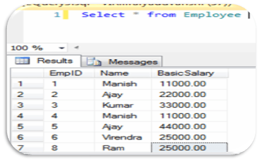
— Create a VIEW on Employee Table
Create View Vw_Employee As
Select * from Employee
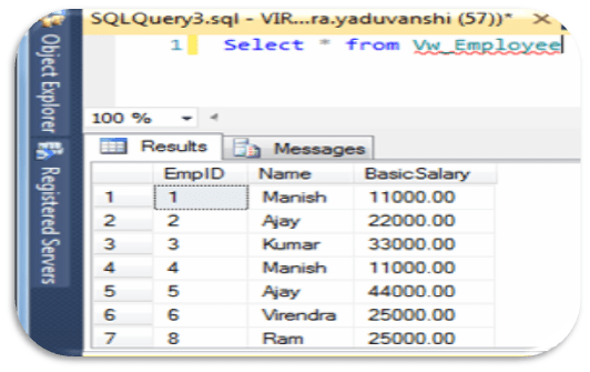
— Lets Check Records from view ‘Vw_Employee’
Select * from Vw_Employee
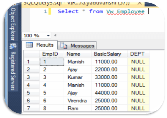
— Now , Add a new column DEPT
Alter Table Employee Add DEPT varchar(20)
— Now Lets Check Records from view ‘Vw_Employee’
Select * from Vw_Employee

Here, you can see, DEPT column not get updated with VIEW
— To resolve the problem / sync columns with base/underlying tables
Execute SP_RefreshView ‘Vw_Employee’
— OR —
Alter View Vw_Employee as
Select * from Employee
Now Lets Check View, its now as per base table.
Now let the worst case, if drop one or more columns and add equal or more number columns to the table then,
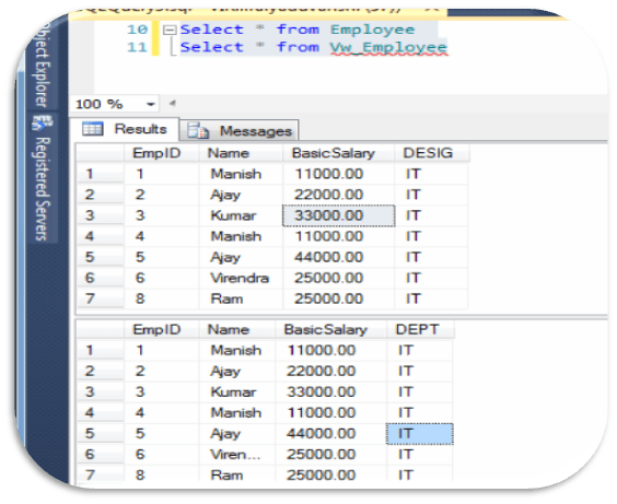
Here, you can see, as per table, View is showing wrong output, and to sync both we have to either run SP_RefreshView or ALTER VIEW command.
Hence, prevention is don’t use wild card “*” while creating VIEWS. But even listing out columns is just a good practice not a solution, it may be even after listing out the columns, if table altered as drop a column from that has been used in VIEW is again same problem.
The permanent solution is creating the view using “WITH SCHEMABINDING” option.
lets, I will explain it in my next blog.
Similarity and Difference between Truncate and Delete
Posted: November 23, 2012 by Virendra Yaduvanshi in Database AdministratorTags: Delete, Delete in SQL Server, Difference Between Delete and Truncate, Similarity and Difference between Truncate and Delete, SQL Server DELETE, SQL Server Truncate, Truncate, Truncate in SQL Server
Similarity
These both command will only delete data of the specified table, they cannot remove the whole table data structure.
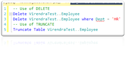
Difference
- TRUNCATE is a DDL (data definition language) command whereas DELETE is a DML (data manipulation language) command.
- We can’t execute a trigger in case of TRUNCATE whereas with DELETE command, we can execute a trigger.
- TRUNCATE is faster than DELETE, because when you use DELETE to delete the data, at that time it store the whole data in rollback space from where you can get the data back after deletion. In case of TRUNCATE, it will not store data in rollback space and will directly delete it. You can’t get the deleted data back when you use TRUNCATE.
- We can use any condition in WHERE clause using DELETE but you can’t do it with TRUNCATE.
- If table is referenced by any foreign key constraints then TRUNCATE will not work.
SP_EXECUTESQL v/s EXECUTE
Posted: November 22, 2012 by Virendra Yaduvanshi in Database AdministratorTags: Difference between sp_executesql and execute, SP_EXECUTESQL v/s EXEC, sp_executesql v/s execute, SP_EXECUTESQL v/s EXECUTE/EXEC, What is the difference between sp_executesql and execute, When to use sp_executesql and execute, which one better sp_executesql or execute
sp_executesql is use for parameterized statements while EXEC does not support Parameterized statements. Parameterized statements is more secured in terms of SQL injection and its better reuse in the plan cache which reduces overhead on the server and boost up performance. Sp_executesql executes a string of Transact-SQL in its own self-contained batch. When it is run, SQL Server compiles the code in the string into an execution plan that is separate from the batch that contained the sp_executesql and its string.
Suppose, if a query which takes a parameter i.e. “EmpID”, When we run the query with ” EmpID ” as 1 and 2 it would be creating two different cache entry (one each for value 1 and 2 respectively).
— First clear Proc cache
DBCC Freeproccache
Go
— Lets Check
— Using EXEC
Declare @strQuery nvarchar(1000)
Select @strQuery = ‘Select * from Employee where EmpID = ”1”’
Exec (@strQuery)
Select @strQuery = ‘Select * from Employee where EmpID = ”2”’
Exec (@strQuery)
— Using SP_EXECUTESQL
–Declare @strQuery nvarchar(1000)
Select @strQuery = ‘Select * from Employee where EmpID =@EmpID’
Exec sp_executesql @strQuery, N’@EmpID int’, 1
Exec sp_executesql @strQuery, N’@EmpID int’, 2
— Lets Check execution count for both
Select sqlTxt.text, QS.execution_count from sys.dm_exec_query_stats QS
Cross Apply (Select [text] from sys.dm_exec_sql_text(QS.sql_handle)) as sqlTxt
It means for Unparameterised (EXEC ) queries the cached plan is reused only if we ask for the same id again. So the cached plan is not of any major use. In case of SP_EXECUTESQL- means for “Parameterised” queries the cached plan would be created only once and would be reused ‘n’ number of times. Similar to that of a stored procedure. So this would have better performance.
sp_executesql works as “Forced Statement Caching” while EXEC works as “Dynamic String Execution”
Summarizing Data with ROLLUP, CUBE, GROUPING SETS, COMPUTE and COMPUTE BY
Posted: November 20, 2012 by Virendra Yaduvanshi in Database AdministratorTags: Avoiding nested queries, Column Name for CUBE, Column Name for ROLLUP, Command for Summarizing Data, COMPUTE and COMPUTE BY, Compute and compute by in sql server, CUBE, CUBE in SQL server, Difference between ORDER BY and the COMPUTE BY, Difference between ROLLUP and CUBE, GROUPING SETS, Grouping Sets in SQL Server, Header for CUBE, Header for ROLLup, How to group data, Query Performance, Query to group Data, Reporting from T-SQL, ROLLUP in SQL Server, SQL Serer, SQL Server Summarizing Data, Summarizing Data commnads in SQL Server, Summarizing Data in SQL Server, Summarizing Data with COMPUTE, Summarizing Data with COMPUTE BY, Summarizing Data with CUBE, Summarizing Data with GROUPING SETS, Summarizing Data with ROLLUP, Summarizing groups of by compute clause, T-SQL Summarizing data Commands
Its very common, The GROUP BY statement to is used to summarize data, is almost as old as SQL itself. Microsoft introduced additional paradigm of ROLLUP and CUBE to add power to the GROUP BY clause in SQL Server 6.5 itself. The CUBE or ROLLUP operators, which are both part of the GROUP BY clause of the SELECT statement and The COMPUTE or COMPUTE BY operators, which are also associated with GROUP BY.
A very new feature in SQL Server 2008 is the GROUPING SETS clause, which allows us to easily specify combinations of field groupings in our queries to see different levels of aggregated data.
These operators generate result sets that contain both detail rows for each item in the result set and summary rows for each group showing the aggregate totals for that group. The GROUP BY clause can be used to generate results that contain aggregates for each group, but no detail rows.
COMPUTE and COMPUTE BY are supported for backward compatibility. The ROLLUP operator is preferred over either COMPUTE or COMPUTE BY. The summary values generated by COMPUTE or COMPUTE BY are returned as separate result sets interleaved with the result sets returning the detail rows for each group, or a result set containing the totals appended after the main result set. Handling these multiple result sets increases the complexity of the code in an application. Neither COMPUTE nor COMPUTE BY are supported with server cursors, and ROLLUP is. CUBE and ROLLUP generate a single result set containing embedded subtotal and total rows. The query optimizer can also sometimes generate more efficient execution plans for ROLLUP than it can for COMPUTE and COMPUTE BY. When GROUP BY is used without these operators, it returns a single result set with one row per group containing the aggregate subtotals for the group. There are no detail rows in the result set.
To demonstrate all these, lets create a sample table as SalesDate as
— Create a Sample SalesData table
CREATE TABLE SalesData (EmpCode Char(5), SalesYear INT, SalesAmount MONEY)
— Insert some rows in SaleData table
INSERT SalesData VALUES(1, 2005, 10000),(1, 2006, 8000),(1, 2007, 17000),
(2, 2005, 13000),(2, 2007, 16000),(3, 2006, 10000),
(3, 2007, 14000),(1, 2008, 15000),(1, 2009, 15500),
(2, 2008, 19000),(2, 2009, 16000),(3, 2008, 8000),
(3, 2009, 7500),(1, 2010, 9000),(1, 2011, 15000),
(2, 2011, 5000),(2, 2010, 16000),(3, 2010, 12000),
(3, 2011, 14000),(1, 2012, 8000),(2, 2006, 6000),
(3, 2012, 2000)
ROLLUP : – The ROLLUP operator generates reports that contain subtotals and totals. The ROLLUP option, placed after the GROUP BY clause, instructs SQL Server to generate an additional total row. Let see the examples as per our TestData from SalesData Table.
Select EmpCode,sum(SalesAmount) as SalesAMT from SalesData Group by ROLLUP(EmpCode)
Will show result as ,

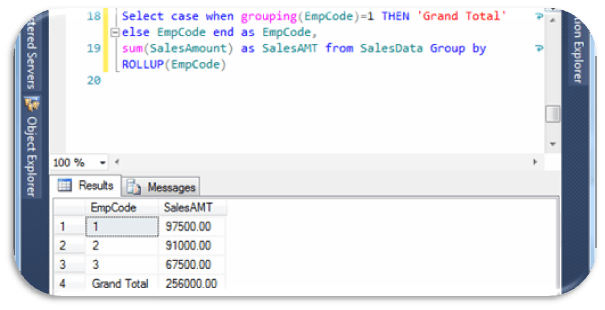
Here we can see clearly sum of all EmpCode with NULL title, Once a guy asked about this NULL , How to give Name for this Null as suppose ‘Grand Total’, here is some manipulation with tricky tips and we can get the desired output and we can also change it as where its required.
Select
case when grouping(EmpCode)=1 THEN ‘Grand Total’ else EmpCode end as EmpCode,
sum(SalesAmount) as SalesAMT from SalesData Group by ROLLUP(EmpCode)
will show result as,
In ROLLUP parameter we can also set multiple grouping set like ROLLUP(EmpCode,Year), hence ROLLUP outputs are hierarchy of values as per selected columns.
CUBE : The CUBE operator is specified in the GROUP BY clause of a SELECT statement. The select list contains the dimension columns and aggregate function expressions. The GROUP BY specifies the dimension columns by using the WITH CUBE keywords. The result set contains all possible combinations of the values in the dimension columns, together with the aggregate values from the underlying rows that match that combination of dimension values. CUBE generates a result set that represents aggregates for all combinations of values as per the selected columns. Let see the examples as per our TestData from SalesData Table.
Select EmpCode,SalesYear,sum(SalesAmount) as SalesAMT from SalesData Group by CUBE(SalesYear,EmpCode)
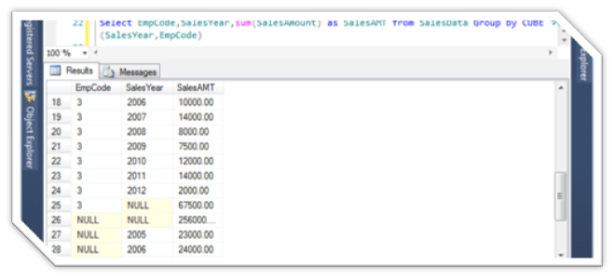
Will shows as
Select SalesYear,EmpCode,sum(SalesAmount) as SalesAMT from SalesData Group by CUBE(SalesYear,EmpCode)
Will show as,
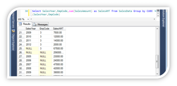
The ROLLUP and CUBE aggregate functions generate subtotals and grand totals as separate rows, and supply a null in the GROUP BY column to indicate the grand total.
the difference between the CUBE and ROLLUP operator is that the CUBE generates a result set that shows the aggregates for all combinations of values in the selected columns. By contrast, the ROLLUP operator returns only the specific result set.The ROLLUP operator generates a result set that shows the aggregates for a hierarchy of values in the selected columns. Also, the ROLLUP operator provides only one level of summarization
GROUPING SETS : The GROUPING SETS function allows you to choose whether to see subtotals and grand totals in your result set. Its allow us versatility as
- include just one total
- include different levels of subtotal
- include a grand total
- choose the position of the grand total in the result set
Let See examples,
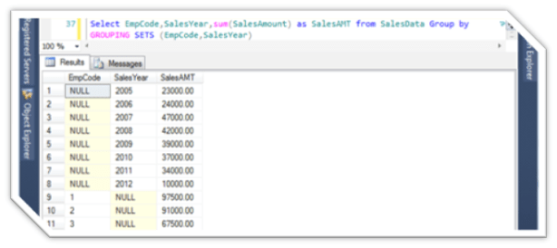
Select EmpCode,SalesYear,sum(SalesAmount) as SalesAMT from SalesData Group by GROUPING SETS (SalesYear,EmpCode)
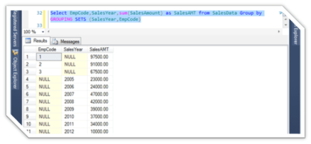
Select EmpCode,SalesYear,sum(SalesAmount) as SalesAMT from SalesData Group by GROUPING SETS (EmpCode,SalesYear)
COMPUTE & COMPUTE BY: The summary values generated by COMPUTE appear as separate result sets in the query results. The results of a query that include a COMPUTE clause are like a control-break report. This is a report whose summary values are controlled by the groupings, or breaks, that you specify. You can produce summary values for groups, and you can also calculate more than one aggregate function for the same group.
When COMPUTE is specified with the optional BY clause, there are two result sets for each group that qualifies for the SELECT:
- The first result set for each group has the set of detail rows that contain the select list information for that group.
- The second result set for each group has one row that contains the subtotals of the aggregate functions specified in the COMPUTE clause for that group.
When COMPUTE is specified without the optional BY clause, there are two result sets for the SELECT:
- The first result set for each group has all the detail rows that contain the select list information.
- The second result set has one row that contains the totals of the aggregate functions specified in the COMPUTE clause.
Comparing COMPUTE to GROUP BY
To summarize the differences between COMPUTE and GROUP BY:
- GROUP BY produces a single result set. There is one row for each group containing only the grouping columns and aggregate functions showing the subaggregate for that group. The select list can contain only the grouping columns and aggregate functions.
-
COMPUTE produces multiple result sets. One type of result set contains the detail rows for each group containing the expressions from the select list. The other type of result set contains the subaggregate for a group, or the total aggregate for the SELECT statement. The select list can contain expressions other than the grouping columns or aggregate functions. The aggregate functions are specified in the COMPUTE clause, not in the select list.
Let See example
Select EmpCode,SalesYear,SalesAmount from SalesData order by EmpCode,SalesYear COMPUTE SUM(SalesAmount)
The COMPUTE and COMPUTE BY clauses are provided for backward compatibility. Instead, use the following components, both are discontinued from SQL Server 2012.
Magic Tables
Posted: November 20, 2012 by Virendra Yaduvanshi in Database AdministratorTags: deleted table in sql server, inserted table in sql server, Magic Table Example, Magic Table example in SQL Server, magic table with example, Magic Tables, SQL Server, SQL Server Magic Table, SQL Server Magic Table Example, SQL Server Magic Tables, Trigger use Magic Table, Trigger's Magic Table, use of magic table or virtual table, virtual table with example
Magic Tables are invisible tables which created on MS SQL Server, during INSERT/UPDATE/DELETE operations on any table. These tables temporarily persists values before completing the DML statements.
Magic Tables are internal table which is used by the SQL server to recover recently inserted, deleted and updated data into SQL server database. That is when we insert or delete any record from any table in SQL server then recently inserted or deleted data from table also inserted into inserted magic table or deleted magic table with help of which we can recover data which is recently used to modify data into table either use in delete, insert or update to table. Basically there are two types of magic table in SQL server namely: INSERTED and DELETED, update can be performed with help of these twos. When we update the record from the table, the INSERTED table contains new values and DELETED table contains the old values. Magic Tables does not contain the information about the Columns of the Data Type text , ntext or image. These are maintained by SQL Server for internal processing whenever an update,insert,Delete occur on table.
These Magic tables is used In SQL Server 6.5, 7.0 & 2000 versions with Triggers only while in SQL Server 2005, 2008 & 2008 R2 Versions can use these Magic tables with Triggers and Non-Triggers also. Magic tables with Non-Trigger activities uses OUTPUT Clause in SQL Server 2005, 2008 & 2008 R2 versions.
Suppose we have Employee table, Now We need to create two triggers to see data with in virtual tables Inserted and Deleted and without triggers.
For INSERTED virtual table, using Trigger ( Magic Tables with Triggers)
CREATE TRIGGER trg_Emp_Ins ON Employee
FOR INSERT
AS
begin
/* Here you can write your required codes, but I am here putting only demostration of Magic Table.*/
Print ‘Data in INSERTED Table’
SELECT * FROM INSERTED — It will show data in Inserted virtual table
Print ‘Data in DELETED Table’
SELECT * FROM DELETED — It will show data in Deleted virtual table
end
–Now insert a new record in Employee table to see data with in Inserted virtual tables
INSERT INTO Employee(Name, BasicSalary) VALUES(‘Virendra’,2000)
For INSERTED virtual table, without Trigger ( Magic Tables with Non-Triggers)
— Use INSERTED Magic Tables with OUTPUT Clause to Insert values in Temp Table or Table Variable
create table #CopyEMP(CName varchar(12),CDept varchar(12))
–Now insert a new record in Employee table to see data with in Inserted virtual tables
Insert into Employee(Name, BasicSalary) OUTPUT INSERTED.Name, INSERTED.BasicSalary into #CopyEMP values(‘Ram’,‘100’)
Select * from #CopyEMP
For DELETED virtual table, using Trigger ( Magic Tables with Triggers)
CREATE TRIGGER trg_Emp_Ins ON Employee
FOR DELETE
AS
Begin
/* Here you can write your required codes, but I am here putting only demostration of Magic Table.*/
Print ‘INSERTED Table’
SELECT * FROM INSERTED — It will show data in Inserted virtual table
Print ‘DELETED Table’
SELECT * FROM DELETED — It will show data in Deleted virtual table
End
–Now Delete few records in Employee table to see data with in DELETED virtual tables
DELETE Employee where BasicSalary > 10000
For DELETED virtual table, without Trigger ( Magic Tables with Non-Triggers)
— Use DELETED Magic Tables with OUTPUT Clause to Insert values in Temp Table or Table Variable
create table #CopyEMP(CName varchar(12),CDept varchar(12))
–Now Delete record in Employee table to see data with in DELETED virtual tables
DELETE Employee where BasicSalary > 10000
Select * from #CopyEMP
Ranking Functions – ROW_NUMBER,RANK,DENSE_RANK,NTILE
Posted: November 19, 2012 by Virendra Yaduvanshi in Database AdministratorTags: DENSE_RANK, How to use SQL Server Ranking Functions, NTILE, RANK, Ranking Functions (Transact-SQL), Ranking Functions – ROW_NUMBER, Ranking Functions DENSE_RANK, Ranking Functions NTILE, Ranking Functions RANK, Ranking Functions T-SQL, ROW_NUMBER, SQL Server Ranking Functions, SQL Server's Ranking Functions
SQL Server 2005 introduced four new ranking functions: ROW_NUMBER, RANK, DENSE_RANK, and NTILE. These functions allow you to analyze data and provide ranking values to result rows of a query. For example, you might use these ranking functions for assigning sequential integer row IDs to result rows or for presentation, paging, or scoring purposes.
All four ranking functions follow a similar syntax pattern:
function_name() OVER([PARTITION BY partition_by_list] ORDER BY order_by_list)
The basic syntax follows.
ROW_NUMBER() OVER ([<partition_by_clause>] <order_by_clause>)
RANK() OVER ([<partition_by_clause>] <order_by_clause>)
DENSE_RANK() OVER([<partition_by_clause>]<order_by_clause>)
NTILE(integer_expression) OVER ([<partition_by_clause>] <order_by_clause>)
Ranking functions are a subset of the built in functions in SQL Server. They are used to provide a rank of one kind or another to a set of rows in a partition. The partition can be the full result set, if there is no partition. Otherwise, the partitioning of the result set is defined using the partition clause of the OVER clause. The order of the ranking within the partition is defined by the order clause of OVER. Order is required even though partition is optional.
ROW_NUMBER: ROW-NUMBER function returns a sequential value for every row in the results. It will assign value 1 for the first row and increase the number of the subsequent rows.
Syntax:
SELECT ROW_NUMBER() OVER (ORDER BY column-name), columns FROM table-name
OVER – Specify the order of the rows
ORDER BY – Provide sort order for the records
RANK: The RANK function returns the rank based on the sort order. When two rows have the same order value, it provide same rank for the two rows and also the ranking gets incremented after the same order by clause.
Syntax:
SELECT RANK() OVER ([< partition_by_clause >] < order_by_clause >)
SELECT RANK() OVER ([< partition_by_clause >] < order_by_clause >)
Partition_by_clause – Set of results grouped into partition in which RANK function applied.
Order_by_clause – Set of results order the within the partition
In the above example, based on the sort order Employee Name, the Rank is given.
The first two rows in the list has same Employee Name, those rows are given same Rank, followed by the rank of next for another set of rows because there are two rows that are ranked higher. Therefore, the RANK function does not always return consecutive integers.
DENSE_RANK: The DENSE_RANK function is very similar to RANK and return rank without any gaps. This function sequentially ranks for each unique order by clause.
Syntax:
SELECT DENSE_RANK() OVER ([< partition_by_clause >] <order_by_clause>)</order_by_clause>
SELECT DENSE_RANK() OVER ([< partition_by_clause >] )
Partition_by_clause – Set of reults grouped into partition in which DENSE RANK function applied.
Order_by_clause – Set of results Order the within the partition
NTILE: NTILE () splits the set of rows into the specified number of groups. It equally splits the rows for each group when the number of rows is divisible by number of group. The number is incremented for every additional group. If the number of rows in the table is not divisible by total groups count (integer_expression), then the top groups will have one row greater than the later groups. For example if the total number of rows is 6 and the number of groups is 4, the first two groups will have 2 rows and the two remaining groups will have 1 row each
Syntax:
SELECT NTILE (integer_expression) OVER ([< partition_by_clause >] <order_by_clause>) </order_by_clause>
SELECT NTILE (integer_expression) OVER ([< partition_by_clause >] )
(integer_expression) – The number of groups into which each partition must be divided.
